Highlight rows in Google Sheets with conditional formatting
I use conditional formatting for individual cells quite a bit. What’s nice is that conditional formatting can also highlight rows in Google Sheets, which is very possible!
Some ways this is useful is when you are analyzing student scores. You can mark rows where the student is proficient in green, where the student is borderline in yellow, and where the students need additional help in red. By being able to highlight rows in Google Sheets with conditional formatting you can look at your data in a more visual way.
For this example, I’ll be using this spreadsheet and when completed, it will show the rows where the student hasn’t turned in the form in red:
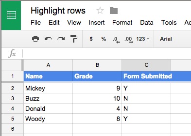
Highlight rows in Google Sheets
I would like it to highlight in red the students who have not turned in their forms. To start, go to Format and select Conditional Formatting… The Conditional format rules panel will display on the right side of the screen:
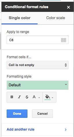
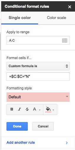
Next, the range to format needs to be set. My data is in columns A through C, so I’ll set Apply to range to A:C. Now to set the Format cells if… In the dropdown, select Custom Formula is. Our custom formula will be the range we want to check and what we want to highlight. This is where it gets tricky. In this example, our formula would be =$C:$C=”N”. Why is that? Let’s break it down:
- = : All formulas start with an equals sign.
- $C:$C : The range we want to compare with “N”. The $ denotes that we want absolute addressing, not relative. This allows us to compare row by row.
- =”N” : We want to compare the contents of the C row and format if it is an N.
Finally, we set the formatting style. Our completed conditional formatting would like like this:
And the spreadsheet now looks like this:
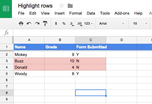
Pretty cool!