Use conditional formatting in Google Sheets to analyze data and grades
Use conditional formatting in Google Sheets to analyze data and grades.

After a formative assessment, you can use a Google Sheet to analyze student performance on individual items on the assessment. This will allow you to spot trends in the students answers, to which you’ll need to investigate what students answered the way they did on individual items. I’m going to show you a quick way of looking at the results in Google Sheets.
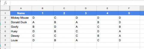
I dumped my hypothetical results of a 5 question multiple choice quiz into Google Sheets. On the left are the student names, and then there is a column for each question.
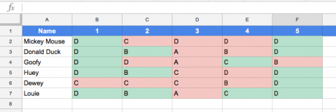
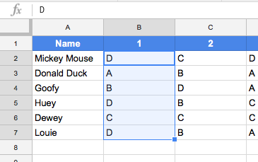
Using conditional highlighting, the correct answer with a green background, and the incorrect answer with a red background, making it easy to see patterns in the results. To get started, highlight the cells which contain the students’ responses to question 1.
Under the Format menu, select Conditional Highlighting.
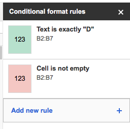
The first conditional format to be applied is the green background for correct answer. In the drop down, select Text is exactly, and in the box put the letter of the correct answer. The correct answer for question one on this hypothetical quiz is D.
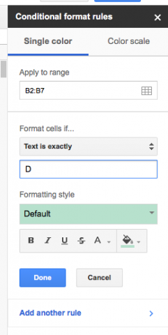
Click Done, and then Add another rule… For this rule, the default condition works for us, but we need to change the background to red.
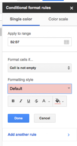
The conditional rules start at the top and stop when they match a ocondition of the cell. The first rule checks for a correct answer, and if it isn’t correct, it moves to the next rule. This only checks whether the cell is empty or not, so it will match the other responses and mark them as red.
Now when we look at the results, we can tell there is something horribly wrong with question three. You would need to go back and look at the question and figure out why none of the students got the question correct.