ⓔ Highlight the minimum and maximum cell in a Google Sheet column #gafetip #itip15

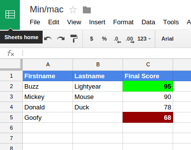
There are times when you are using a Google Sheet, such as collecting information in a form, where you would like highlight the minimum and maximum cell in a column. Google Sheets offers conditional formatting, which gives you the ability to change the formatting of a cell based on the contents of the cell. For the minimum and maximum, we are going to apply conditional formatting to an entire column.

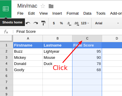
First, select the column by click on the column header for the column:

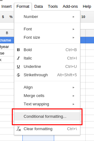
Under the Format menu, select Conditional Formatting…

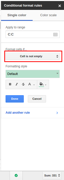
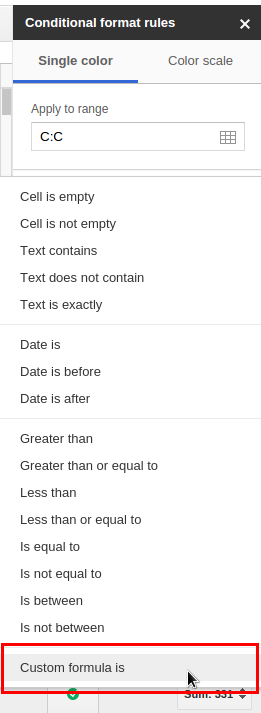
The Apply to range will already be filled in with the currently selected range. The magic happens under Format cells if… Click Cell is not empty and select Custom formula is… from the list:

 

 

 

 

 

 

 

 

 

 

 

 

 

 

 

 

In the Value or Formula  box you will be entering the formula. We will use the min() function first. Entering the formula will look a little different, because we have to use absolute reference to the range so the min() function will work. Our formula will look like this: =$C:$C=min(C:C):

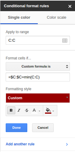
Pretty different to how we normally use formulas, but hey, it works. Select the formatting you want to apply to the minimum value. Something like a red background with white letters stand out.

Now click Add another rule…

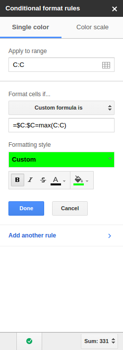
And replace min in the function with max, and update the colors (maybe something green):

Hit done  and, voilà, Google Sheets will now highlight the minimum and maximum cell in a column!