Color grades in a Google Sheet faster with a color scale
I’ve talked about using conditional formatting in the past, setting different grade ranges to different colors. The results are good, but the prep time is tedious. There is a faster way, conditional formatting with a color scale!
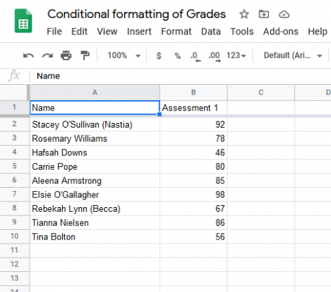
Take this:
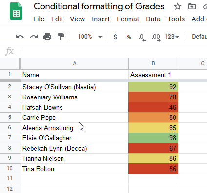
And turn it in to this:
To try it out, get the data in your Google Sheet. Click on the column you want to color scale and select conditional formatting.
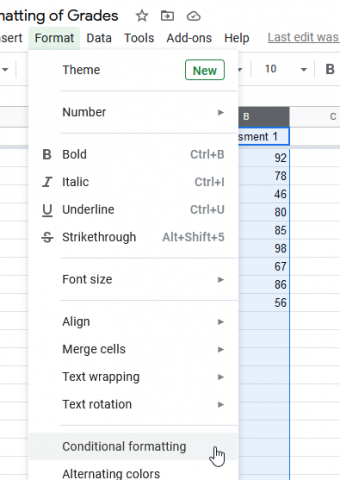
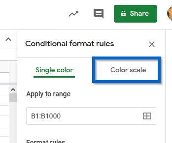
Then click on Color Scales:
The default rules will make the lowest grade come in dark green, and the highest grade in white. 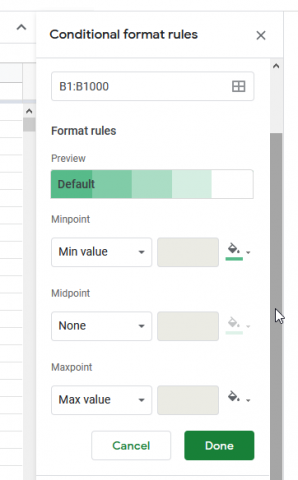
We can do better than that. Here I changed the lowest to red, so anything lower than 60 was red. Midpoint is 80, and that’s yellow. The highest is 100, and that’s green.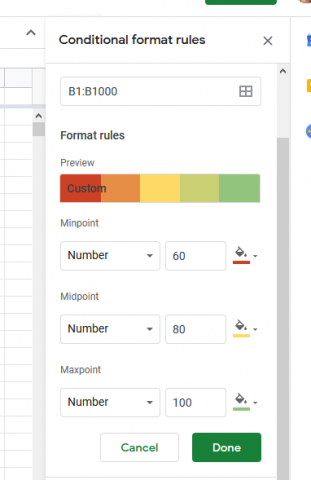
So now, I can look at the grades and see exactly who needs help.
The scale can also go on percentages, and you can play with the min, mid, and max points for the scales. Check out my example sheet and play around!